Estimating True Infections: A Simple Heuristic to Measure Implied Infection Fatality Rate

By: Youyang Gu
July 29, 2020

Table of Contents

• Main Conclusions
• Introduction
• Disclaimers
• Data
• Prevalence Ratio
• Using Confirmed Deaths
• Putting it Together
• Implied Infection Fatality Rate (IIFR)
• Distribution of Infections by Age
• Discussion
  • Relationship between Positivity Rate and Prevalence Ratio
  • Higher Infections in July
  • Lower IIFR Over Time
  • Effective Herd Immunity
• Conclusion

November 2020 Update: We have released a revised version of this report based on new data and research since the original published date (July 2020).

Important: While this page explains how one can use cases and positivity rate to estimate true infections, our covid19-projections.com model only use deaths data.

November 2020 Update: As testing continues to increase across the United States, we want to caution readers from applying the below formulas to the new fall data. The findings below are more relevant during the period when testing was limited, and may no longer be as applicable since the summer. In addition, please read this article by the COVID Tracking Project that highlights the difficulty of computing consistent test positivity rates.

August 10 Update: See our new findings for a case study regarding the role of immunity, behavior, and interventions in the spread of COVID-19.

Main Conclusions

• Infections are more prevalent in June/July (peak of ~450,000 new infections per day) than in March/April (peak of ~300,000 new infections per day). This is likely driven by reopenings, a lack of policy intervention, and a more widespread prevalence of the virus. The rest of this page describes our methodology for deriving this estimate, with more discussion below.
• Implied infection fatality rate (IIFR) dropped from 1% in March to 0.6% in May to 0.25% in July. This is likely primarily driven by a lower median age of infection. Improved treatments, better protection of vulnerable populations, earlier detection, and virus seasonality also likely contribute to a lower fatality rate. See our section on IIFR below, along with further discussion.
• Infections in high-impacted states began to slow down after reaching 10-35% population prevalence. It is likely that this is a result of regions reaching a certain degree of effective herd immunity that is suppressing further spread. This threshold may be lower in June/July than it was in March/April, which is expected since the effective reproduction number, Rt, is now much lower. Reaching this temporary effective herd immunity threshold does not stop transmission - it simply slows down further transmission. Changes in human behavior and policy interventions such as mask mandates also contribute to a slowing of the spread. If current interventions and social distancing are relaxed, or if immunity is lost over time, then it is possible that we will see another increase in the rate of transmission. More discussion and caveats below.

Summary and discussion on Twitter

Introduction

Knowing the true number of people who are infected with COVID-19 in the US is an essential step towards understanding the disease. But estimating this number is not a simple task. The true number of infections is many times greater than the reported number of cases in the US because the majority of infected individuals do not get tested due to several reasons: 1) they are asymptomatic, 2) they are only mildly symptomatic, 3) they do not have easy access to testing, or 4) they simply do not want to.

On this page, we introduce a simple square root function to estimate the true prevalence of COVID-19 in a region based on only the confirmed cases and test positivity rate: true-new-daily-infections = daily-confirmed-cases * (16 * (positivity-rate)^(0.5) + 2.5). We will also introduce the implied infection fatality rate (IIFR), which is a metric derived by taking a region’s reported deaths and dividing it by the true infections estimate (after accounting for lag).

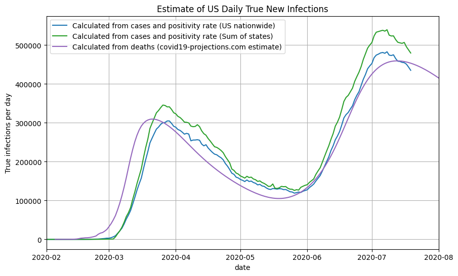
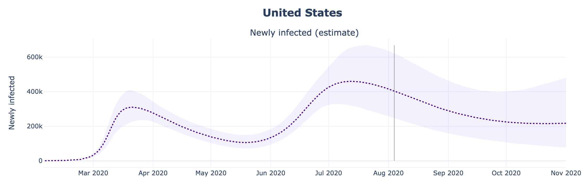
Using this method, we estimate that the true number of new infections peaked at close to 500,000 new infections per day in July, compared to 300,000 new infections per day in March. This means that the peak of infections after reopening is 60% higher than the initial peak in March. In total, by the end of July 2020, we estimate over 35 million (1 in 10) Americans have been infected at some point by the SARS-CoV-2 virus.

Below, you can see a plot of our infection estimates for the US. We compare the results to the covid19-projections.com model, which uses only past reported deaths to estimate the number of true infections.

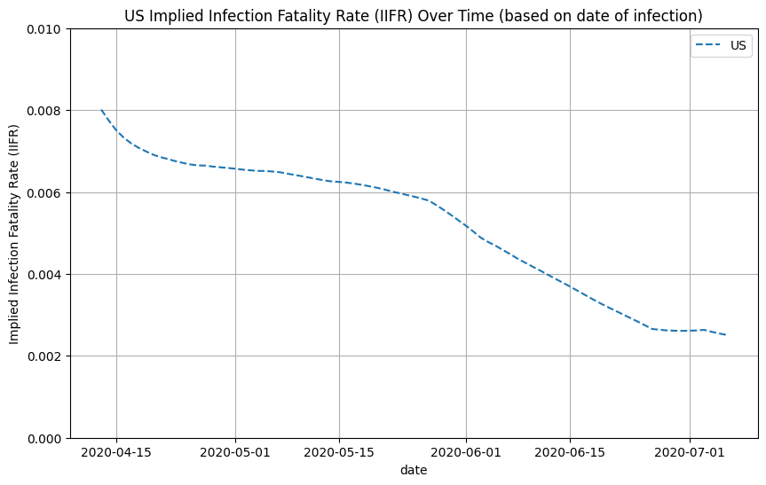
Once we have a reasonable estimate of the true number of newly infected individuals per day, we can use the reported deaths to compute the implied infection fatality rate (IIFR). The IIFR for the US was above 1% in March, stabilized at around 0.6% in April-May before decreasing to ~0.25% in July. Note that our IIFR estimate does not take into account excess/unreported COVID-19 deaths, so it is likely a lower bound for the true IFR. This is further explained below.

Disclaimers

• All of the work presented on this page has not been peer-reviewed, and so we encourage reading this with a healthy dose of skepticism. We hope that the reader can make their own conclusions based on the evidence we present. This is just one possible take on the situation, and the results are subject to change based on new data/evidence.

• Note that our use of the term infection fatality rate (IFR) refers to true deaths divided by true infections. It is not age-adjusted. As a result, if there is an increasing prevalence of the disease in a younger population, then the IFR will decrease, despite the deadliness of the virus remaining unchanged among a particular age group. It is likely that the fatality rate for a given age group have not changed significantly.

• To compute our estimates of the implied infection fatality rate (IIFR), we use only reported deaths in the numerator. If a state is significantly underreporting COVID-19 deaths, then our estimates will likely underestimate the true IFR. Since most states are underreporting COVID-19 deaths, our IIFR estimate is closer to a lower bound for the true infection fatality rate. For example, if true deaths is 50% higher than reported deaths, then the true IFR will be roughly 50% higher than the IIFR. To get a better understanding of the true deaths caused by COVID-19, we recommend looking into excess deaths, something we do not do in this analysis.

• Our usage of the “herd immunity threshold” is not necessarily rigorous, as the term is traditionally used in the context of long-term immunity obtained by vaccination. We believe there should be a better term to describe the current phenomenon where transmission is slowed as a result of social distancing and people gaining temporary immunity. If social distancing measures are relaxed and/or immunity is lost over time, then it is possible that transmission will increase again. Hence, the term “herd immunity” may be misleading.

• As states expand their testing capacity and make testing more accessible for everyone, it is possible that the relationship we present on this page becomes less relevant. We provide possible explanations for this in the Discussion.

• The outputs from this analysis are only as good as the provided input data. If states, for example, underreport/misrreport COVID-19 deaths, then that could significantly skew the outcome of this analysis. Hence, we call on all states to follow national guidelines and report data in a honest, comprehensive, and consistent manner.

• This approach was optimized on US data. It is not necessarily applicable to countries outside the United States, where testing guidelines/procedures may be drastically different. One may need to refit the prevalence curve to suit each country.

• While all the methods on this page were developed independently, we want to note that this is not a novel approach. See prior work by Peter Ellis, David Blake, and Campbell et al.

Back to Top

Data

Input: For this report, we use reported cases and deaths data from Johns Hopkins CSSE and testing data from The COVID Tracking Project.

Output: We have uploaded the infections estimates and implied IFR calculations to our GitHub. You can find the daily summary here. We aim to update those files daily. Currently, we only have IIFR estimates for the US. We are working to expand this concept to other countries.

Note: The above inputs and outputs are only used for the purpose of this report. Our modeling work is completely separate, and only uses daily reported deaths from Johns Hopkins.

Back to Top

Prevalence Ratio

The core idea behind this method is that we can use the positivity rate to roughly determine the ratio of true infections to reported cases. The hypothesis is that as positivity rate increases, the higher the true prevalence in a region relative to the reported cases. This also makes sense intuitively: if you test everyone, then the positivity rate will be very low, and you will catch every case. But if testing is not widely available, then you will catch only the severe cases, resulting in a higher positivity rate. This phenomenon is sometimes referred to as preferential testing.

We believe that the relationship between positivity rate and ratio of true prevalence is monotonically increasing. Of course, the exact relationship varies from state to state and across time. But if one were to take the average across all of the data, one can generate a theoretical curve. We believe this relationship can be approximated by a root function of the following form:

prevalence-ratio = a * (positivity-rate)^(b) + c

where a, b, c are unknown constants.

Through curve fitting on historical test positivity and seroprevalence surveys, as well as trial & error, we found that the following square root approximation function works well:

prevalence-ratio = 16 * (positivity-rate)^(0.5) + 2.5

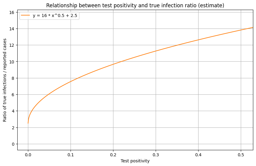
To see if this relationship passes the “common sense test”, we can take a look at the US positivity rate over time (below). In March/April, the US positivity is around 20%, which corresponds to a prevalence ratio of roughly 10x the number of reported cases when using the function above. This seems to be a reasonable estimate, and matches estimates provided by the CDC. In New York and New Jersey during this period, test positivity was around 40-50%, which corresponds to a roughly 12-15x prevalence (later substantiated by serology surveys). In June, when US positivity is around 5%, the function estimates a prevalence of roughly 6x the number of reported cases, which seems reasonable. We use a y-intercept of 2.5 to indicate minimum prevalence ratio of 2.5x to account for asymptomatic individuals.

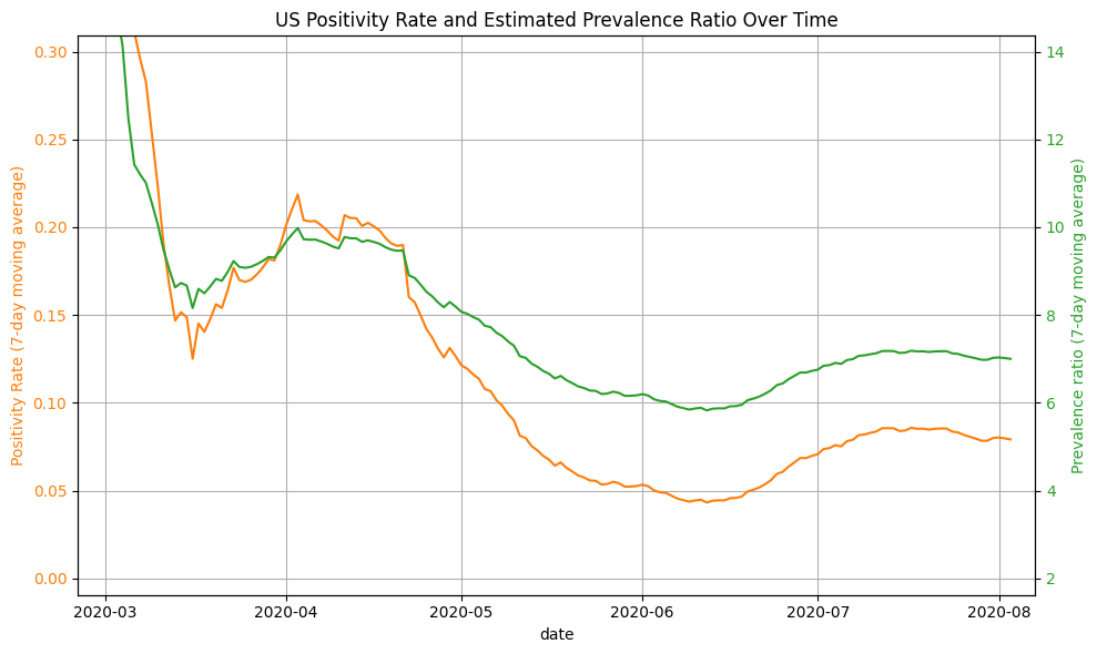
The next step is to map all reported cases to true new infections based on the true prevalence ratio. We can compute the true prevalence ratio simply by inserting the positivity rate into the function above. We then multiple the ratio by the daily confirmed cases to get the true daily infections:

true-new-daily-infections = daily-confirmed-cases * prevalence-ratio

For all computation purposes, we use the 7-day average of confirmed cases and positivity rates. Combining the two functions from above, we get:

true-new-daily-infections = daily-confirmed-cases * (16 * (positivity-rate)^(0.5) + 2.5)

As an example, let’s say that the US reported 67,000 new cases with a 8.5% positivity rate on July 22. This would result in a true prevalence ratio of 16*sqrt(0.085)+2.5 = 7.16. We can then multiply this ratio by the confirmed cases to get the true new infections. In this example, we estimate there to be 7.16 * 67,000 = ~480,000 true new infections. Because reported cases lag infections by roughly 2 weeks, we must shift the result back by two weeks. So the 480,000 true infections actually took place approximately 14 days before July 22, on July 8.

Back to Top

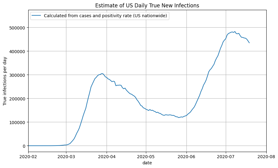
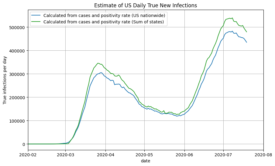
Using US Nationwide Cases + Positivity Rates

For US nationwide data, we can compute the true prevalence ratio by passing in the daily positivity rate to our approximation function above. We then multiply the true prevalence ratio by the number of confirmed cases each day to get the number of true new infections. Note that all daily numbers used are 7-day moving averages. Finally, we shift the true new infections back by 14 days to account for reporting delays. We can now plot the results as a function of the date:

Using State-by-state Cases + Positivity Rate

Rather than using the US nationwide cases and positivity rates, we can use the state-by-state cases and positivity rates to compute the true new infections for each state using the same method described above. Below is a plot of the estimated true daily new infections for a selection of states. Using this approach, you can see that Florida and Texas are nearing the maximum daily new infections set by New York back in March.

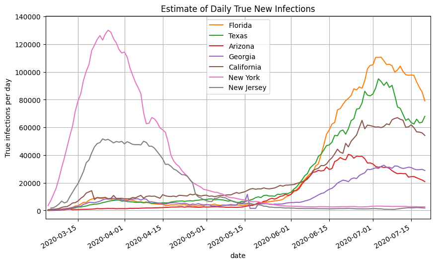
We then take the sum of the infections estimates for all 50 states and territories to get the nationwide daily new infections (orange line). Note that it closely aligns with the graph generated using the US nationwide data.

Back to Top

Using Confirmed Deaths

We can compare the previous approach to a method used by covid19-projections.com. It uses only past reported deaths to predict future reported deaths. You can read more about our model here.

One of the outputs generated by our model is the number of true infections in each region and country. We simply take that output from our model to get our estimate of true infections in the US.

Back to Top

Putting it Together

We can now plot all the methods we described above together and see how they compare. Note that they follow roughly the same shape and magnitude.

We offer explanations for some of the minor differences below:

• Estimates using cases vs deaths - shift - On average, cases were detected earlier in June/July compared to March/April. In our current estimates, we assume a constant lag time between a new infection and a reported case. As a result, compared to estimates generated by only deaths data, the plot of infections based on reported cases lag in March/April and lead in June/July. If we used a non-static shift between confirmed cases and new infections (i.e. longer shift in March/April and a shorter shift in June/July), then this difference would be dramatically reduced.
• Estimates using cases vs deaths - magnitude - As testing becomes more widely available in June/July, using this method to estimate true infections may result in an over-estimate of the prevalence ratio in a region. As a result, you can see a larger difference in the difference in peak magnitude when compared to case estimates generated using on deaths. See the Discussion for further explanations.
• Estimates using state-by-state cases vs US nationwide cases - Using state-by-state estimates of positivity rates and cases (rather than nationwide estimates) leads to a slight overestimate in the number of true infections in June/July. We suspect this is partly because of some states (such as Florida, Arizona, Georgia) undercounting the number of negative test results, which artificially inflates the positivity rate and thereby the prevalence ratio. If that factor is adjusted, it is likely that the peaks will line up at slightly over 400,000 new infections per day.

Back to Top

Implied Infection Fatality Rate (IIFR)

We can use these estimates of true infections to compute the implied infection fatality rate (IIFR) for the US by taking the reported deaths from 28 days into the future (7-day moving average) and dividing it by the true infections (7-day moving average). Note that we assume that reported deaths is roughly equal to true deaths. If there is a significant amount of excess/unreported COVID-19 deaths, then our IIFR estimate will be an underestimate of the true IFR. See work from the Weinberger Lab for their analysis of excess deaths.

We can also do this on a state-by-state basis. See below for IIFR plots for select states.

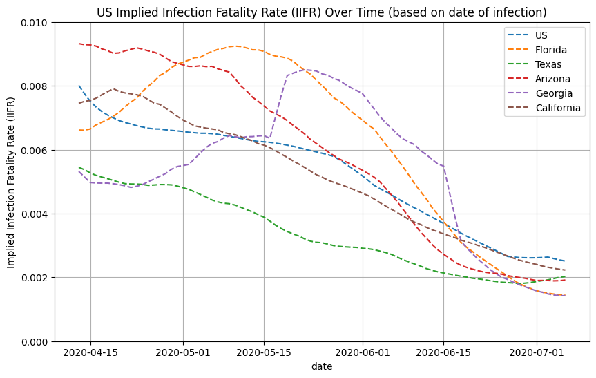
Distribution of Infections by Age

Using CDC’s COVIDView Data that breaks down testing by age, we can see that the median age of confirmed cases has decreased from April to June:

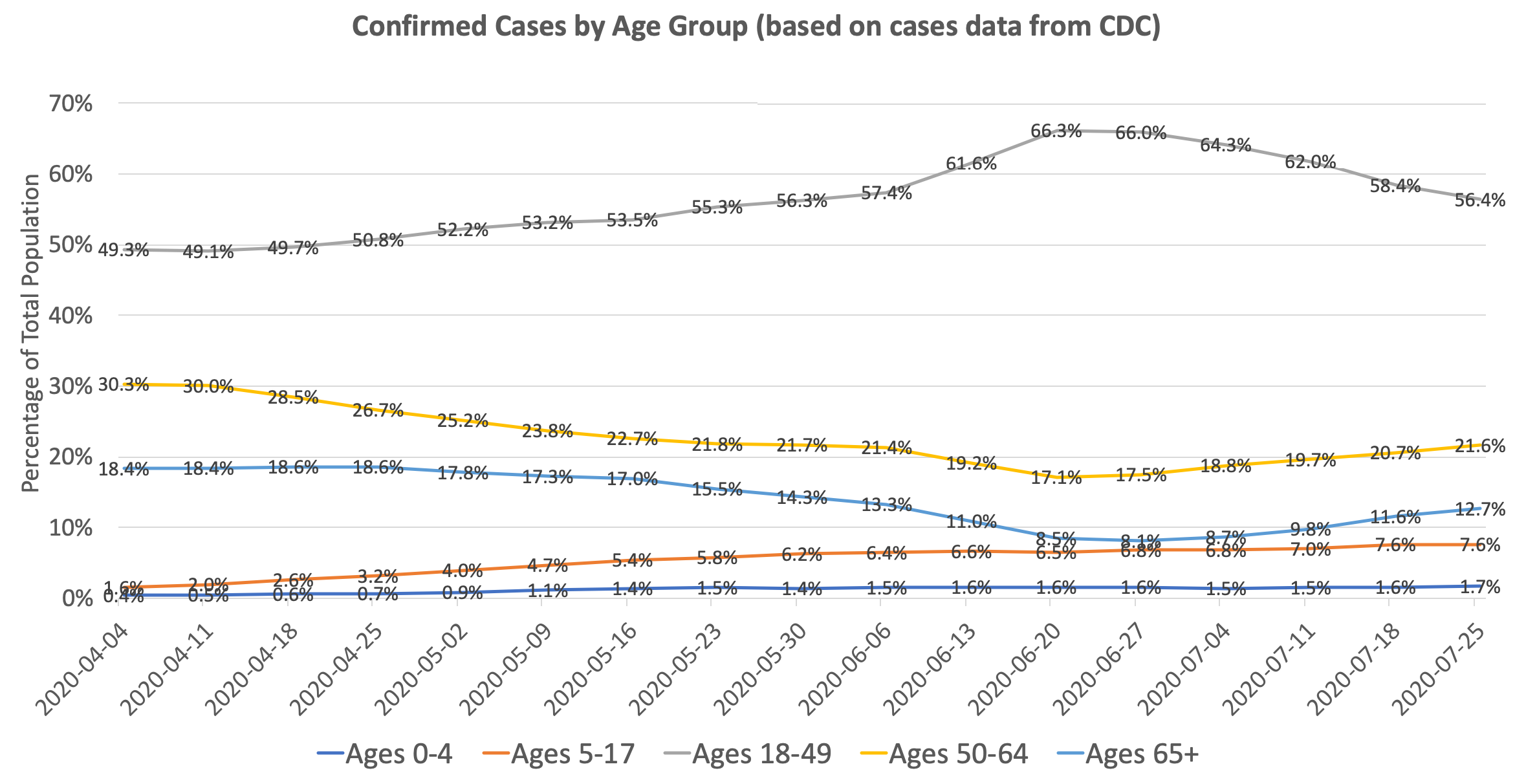
Of course, there can be selection bias on how different age groups are getting tested. One can argue that the reason there is a higher proportion of older people in March/April relative to June/July is because testing was limited, and hence older individuals were prioritized for testing. So one would expect that older age groups have a lower positivity rate than the younger age groups (since you are catching more cases). But if you look at the data, the opposite is true: in March/April, the older age groups actually had a higher positivity rate than the younger age groups. By our prevalence ratio calculation above, this indicates that the prevalence is actually even higher in the older age groups than the younger age groups. This trend was reversed starting in late April, and now younger age groups have a higher positivity rate than older age groups.

We can use our prevalence ratio formula from above to estimate the proportion of true infections by age group given the number of confirmed cases and test positivity rates:

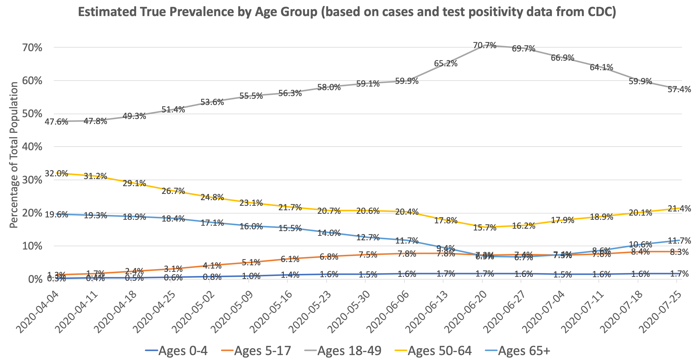
You can see that the change in distribution from old to young is even more pronounced after accounting for test positivity. The ratio of prevalence in individuals ages 18-49 to prevalence in individuals ages 65+ went from roughly 2.5x in April to 10x in June. Since the infection fatality rate in those age 65+ is roughly 10-50x that of those ages 18-49, it’s no surprise that the overall infection fatality rate in the US dropped significantly between March and July. The IFR is further lowered by improving treatments and earlier detection.

As an addendum, the above chart can also explain why reported deaths in the US continued to fall through June despite an increase in cases: the increase in cases is largely driven by younger people with a low infection fatality rate. Unfortunately, the pattern in July indicates that the age distribution of infections is reverting back towards a higher median age of infection, resulting in a sharp spike in deaths in late July/early August. This will likely lead to an increase in the implied infection fatality rate in August and beyond, and is something that we will be monitoring.

Back to Top

Discussion

Relationship between Positivity Rate and Prevalence Ratio

We developed the constants for the prevalence function (prevalence-ratio = a * (positivity-rate)^(b) + c) through a combination of trial & error and curve fitting. We don’t believe this function is perfect. There can be other constants a, b, and c that may be a closer approximation of the true relationship. Because there is no “truth” value to fit the function against, we decided it is not worth trying to perfectly fit this function. As a result, we settled on a simple square root function to describe the relationship.

The exact relationship between positivity rate and prevalence ratio may be different from state to state and across time. Here is a partial list of possible factors that can cause these differences:

• Availability of testing - the greater the number of tests performed (as a percentage of the population), the less the undetected prevalence ratio becomes, and the less the role of positivity rate becomes. See paper by Burger & McLaren for a more in-depth view.
• Differences and changes in reporting guidelines
  • Counting repeated positive tests (skews positivity up)
  • Counting repeated negative tests (skews positivity down)
  • Not reporting all positive tests (skews positivity down)
  • Not reporting all negative tests (skews positivity up)
  • Only reporting Electronic Laboratory Reporting (ELR) tests (skews positivity up)
  • Mixing serology tests with PCR (skews positivity up)
• Backlog of test results - positive tests receive priority for processing, which may skew the positivity rate upwards
• Delay/lag in test results - if tests take 1-2 weeks to be reported, then it may no longer be an accurate representation of how new infections are changing
• Shifting age demographics - Test positivity rates are higher in younger age groups. So a lower median age of infection may also result in a higher positivity rate, causing a possible confounding factor.

For example, here is a story from the Tampa Bay Times that explores how positivity rate is reported in Florida. Meanwhile, Georgia has a different set of standards for test reporting. These guidelines are specific on a per-state level and may differ significantly between states, making comparison more difficult.

We believe that a high positivity rate in June/July implies a lower prevalence ratio than back in March/April, when testing was not as widely available. As a result, future extensions of this work could involve time-dependent prevalence ratio functions, such as a separate functions for March/April and post-April. We think a lower exponent and coefficient may be a better approximation for post-April (e.g. prevalence-ratio = 10 * (positivity-rate)^(0.4) + 2.5).

Back to Top

Higher Infections in July

There are many explanations as to why there are more infections in June/July than in March/April. One reason is based on simple math regarding exponential growth. We started from 0 infections in February with an R0 of ~2.5. There was only a limited period of exponential growth before people began social distancing in March, which quickly brought the Rt value under 1. The stay-at-home orders in most parts of the US were timely and effective in containing the spread and preventing further uncontained spread.

In contrast, when states reopened in May/June, there were already ~100k new infections per day. With an Rt of ~1.2 and limited intervention to mitigate the spread, new infections were able to climb to 400k+ per day in a period of two months. In layman terms, we started from a much higher point in May and had a longer period of time to reach the peak.

Back to Top

Lower IIFR Over Time

The IIFR in the US decreased from over 1% in March to 0.25% in July. Below, we present a few explanations to why the IIFR in the US has decreased significantly since March/April.

• Lower median age of infection (see section above)
• Better protection of vulnerable populations (nearly half of COVID-19 deaths in March/April were in care homes)
• Improved treatment (new drugs, better allocation of resources, more experience among staff, etc)
• Earlier detection
• Seasonality

The above are explanations that would explain a true decrease in IFR. We believe the lower median age of infection and better protection of high-risk populations are the primary drivers behind the decrease in IIFR. Below are some reasons that could skew the IIFR lower, but not change the true IFR:

• More comprehensive reporting of confirmed cases
• Changes in the distribution of age groups tested (e.g. more young people getting tested would skew IIFR down)
• Inflation of the test positivity rate (e.g. double-counting positives, not reporting negatives, etc)
• Longer lag in death reporting
• Underreporting of deaths

Back to Top

Effective Herd Immunity

The term “herd immunity threshold” is traditionally used in the context of long-term immunity obtained by vaccination, but is now frequently being used in the context of COVID-19. We want to be clear that any references to “herd immunity thresholds” in the context of COVID-19 can potentially be misleading, because a removal of current social distancing measures and a loss of immunity over time may cause a resurgence in transmission, despite a region having reached some form of “herd immunity” in the past.

Similar to how the term effective reproduction number measures the reproduction number, Rt, at a certain point in time, we are denoting the term effective herd immunity threshold (eHIT) to mean the herd immunity threshold under the social distancing standards and policy interventions at a given time. This is the minimum percentage of the population immune at a certain time such that transmission slows down under those conditions. If immunity is lost or restrictions are relaxed, then the eHIT may increase.

Looking at the data, we see that transmissions in many severely-impacted states began to slow down in July, despite limited policy interventions. This is especially notable in states like Arizona, Florida, and Texas. While we believe that changes in human behavior and changes in policy (such as mask mandates and closing of bars/nightclubs) certainly contributed to the decrease in transmission, it seems unlikely that these were the primary drivers behind the decrease. We believe that many regions obtained a certain degree of temporary herd immunity after reaching 10-35% prevalence under the current conditions. We call this 10-35% threshold the effective herd immunity threshold, eHIT.

A basic method to calculate standard the herd immunity threshold (HIT) is to use the basic reproduction number, R0: HIT = 1 - 1/R0. Back in March/April, we estimate R0 in the US to be around 2.3. This corresponds to a HIT of 1-1/2.3 = ~0.6, or 60%. But the effective reproduction number, Rt, has decreased dramatically since then due to a variety of reasons such as greater population awareness, mask-wearing, reduced larger gatherings, and implementation of social distancing guidelines. The Rt in most regions around the US where there are outbreaks is now between 1.1-1.6. This corresponds to an effective herd immunity threshold (eHIT) of 10-35%. As a result, it makes intuitive sense that we are seeing a decline in transmission after those regions reach a 10-35% prevalence.

The above method is a very crude method to compute herd immunity thresholds. See paper by Aguas et al. for a better analysis of herd immunity thresholds for SARS-CoV-2 and the effects of population heterogeneity.

One thing to note is that original definition of the herd immunity threshold is derived from the basic reproduction number, R0, and assumes no intervention and no social distancing. Hence, by definition, the HIT of the SARS-CoV-2 virus remains unchanged over time, between 50-80%. But the effective herd immunity threshold (eHIT) in the context of COVID-19 is changing over time because the effective reproduction number, Rt, decreases as a result of society adjusting to the virus. That’s why we are seeing infections and cases plateau and decline after prevalence reaches 10-35% as people gain temporary immunity. A removal of current restrictions and interventions, as well as a loss of immunity over time, may cause this threshold to return to its original levels of 50-80%.

Lastly, note that reaching the effective herd immunity threshold does not stop transmission - it simply slows down further transmission.

Back to Top

Conclusion

To conclude, we presented a simple heuristic that estimates the true prevalence of COVID-19 infections in a region. We also introduced the implied infection fatality rate (IIFR) that estimates the fatality rate as implied by the reported deaths and true prevalence.

Using this methodology, we found that the prevalence is higher in the US during June/July (peak of ~500,000 infections/day) than in March/April (peak of ~300,000 new infections/day). However, the implied fatality rate is significantly lower in June/July (~0.25% IIFR) than in March/April (~1% IIFR).

While this is by no means a comprehensive study, we hope this work can help other scientists and researchers better understand the changing dynamics of this disease over time.

The data and results used on this page can be found on GitHub.