COVID-19 Death Forecasting - Model Details
Note: This write-up is specifically for our death forecasting model that made daily predictions from April to October 2020. For other model variations, see our About page.
For those who prefer a visual medium, you can view Youyang’s August 2020 talk about the model here.
SEIR Model
Our COVID-19 prediction model has an underlying simulator based on an elaboration of the classic SIR model used in epidemiology: the SEIR (susceptible-exposed-infectious-recovered) model. We added an exposed (E) period due to the reported incubation period of COVID-19 during which individuals are not yet infectious.
The SEIR component of our model is open source.
To quickly summarize how an SEIR model works, at each time period, an individual in a population is in one of four states: susceptible (S), exposed (E), infectious (I), and recovered (R). If an individual is in the susceptible state, we can assume they are healthy but have no immunity. If they are in the exposed state, they have been infected with the virus but are not infectious. If they are infectious, they can actively transmit the disease. An individual who is infected ultimately either recovers or dies. We assume that a recovered individual’s chances of re-infection is low, but not zero. We can model the movement of individuals through these various states at each time period. The model’s exact specifications depend on its parameters, which we describe in the next section.
For our SEIR implementation, we use a discrete-time state machine where each step is a day in the simulation. For each day, we have a probability distribution for which individuals in each S/E/I/R state may transition to another S/E/I/R state. For example, we have a probability distribution for when a currently-infected individual will transmit the virus, and another probability distribution for when an infected individual will succumb to the disease. These distributions are then convolved with the total existing cases to determine the number of new infections and new deaths per day. For new infections, we multiple the convolution by R0, while for deaths, we multiple the convolution by the mortality rate.
Assumptions
Please see the About page to read about the assumptions in our model.
Data
The sole data source we use is the daily reported deaths from Johns Hopkins CSSE. In addition, we use population data for each state/country to calculate the total susceptible population.
Because the raw data may be noisy, we must first run a smoothing algorithm to smooth the data. For example, if a state reports 0 death on one day and 300 deaths the next day, we smooth the data to show 150 deaths on each day.
Parameters
For our SEIR model, there are basic inputs/parameters that must be set to begin simulation. Gabriel Goh’s Epidemic Calculator or University of Basel’s covid19-scenarios.org provide good visualizations of sample inputs/parameters into a simulation. We chose a set of parameters that we think are important for the accuracy of the simulation. We divide the parameters into two categories:
Category 1: Fixed parameters
Fixed parameters are those that are fixed for this particular COVID-19 epidemic and likely do not fluctuate significantly across countries/states/regions. These include the following:
- Latency period
- Infectious period
- Time between illness onset to hospitalization
- Time between illness onset to death
- Hospital stay time
- Time to recovery
We use various reports and publications to determine the best values for these fixed parameters. Most of these sources reference studies from Wuhan, China, where the epidemic first began in December 2019. While it is possible that the exact values may fluctuate slightly from region to region, we believe that the impacts these fluctuations have are minimal compared to the variable parameters.
Category 2: Variable parameters
Variable parameters are those that may change depending on the country/state/region. Some examples are the following:
- R0 - the basic reproduction number
- Mortality rate
- Imports of positive cases per day
- Mitigation effects (i.e. post-mitigation R)
- Lockdown fatigue factor
- Lifting of shelter-at-home orders (i.e. post-reopening R)
- Population
While the population of a region can be easily looked up, the other variable parameters are not easily retrievable. We will allocate the majority of our resources towards estimating the most sensible values for these parameters for each region.
Modeling the R value
To model the effects of mitigation strategies such as shelter-at-home/lockdown orders, we use three different R values in our model:
1) R0: the initial R before mitigation strategy 2) post-mitigation R: the R after mitigation strategy 3) post-reopening R: the R after mitigation strategy has been relaxed
Note that the mitigation strategy can encompass a wide variety of strategies, ranging from a complete lockdown as we’ve seen in Wuhan, China, to a more relaxed strategy as we’ve seen in Sweden.
These R values are unknown ahead of time, and will be learned by the model. We use an inverse logistic function to model the transition between R0 and post-mitigation R. We chose the inverse logistic function based on subway ridership data from New York City and California. The shift and the slope of this function is also learned based on the data. For example, we learned that the downward slope of the inverse logistic function is steeper in New York than in Sweden, which matches our intuition that New Yorkers began social distancing at a quicker pace.
We assume that the post-reopening R is greater or equal to the post-mitigation R.
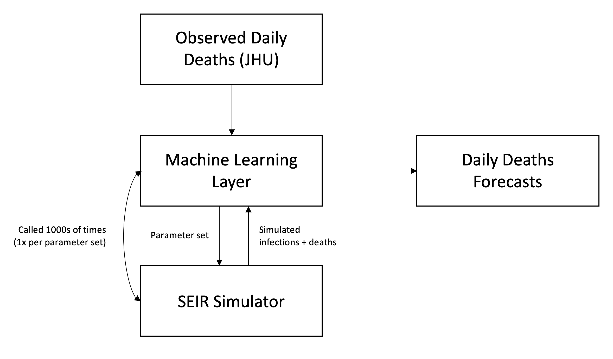
Parameter Search using Machine Learning
As described in the previous section, determining the best values for variable parameters such as R0, the mortality rate, post-mitigation R, and post-reopening R will help us determine how COVID-19 will progress in a region. If we know what the “true” values of those parameters are, we can accurately simulate what is happening in the real world using our SEIR model. To determine these values, we use a simple machine learning technique called grid search.
Parameter Optimization
We found that a brute-force grid search method that iterates through the entire parameter space is the most effective in finding an optimal set of parameters. So if we have 10 values for R0 and 10 values for the mortality rate, then there are 100 different parameter combinations for those two parameters. To optimize computation time, we prune unrealistic parameters (e.g. R0 > 10).
For parameters where we do not have the data to estimate (e.g. we do not know the post-reopening R for regions that have not reopened), we consider all values equally, resulting in a wider confidence interval.
Loss Function
To measure the error of a parameter set, we use a loss function that minimizes the error between our projected daily deaths and the actual daily deaths. We tried various loss functions such as mean squared error, absolute error, ratio error, and an ensemble of the aforementioned errors. We find that the mean squared error loss function consistently performs well on out-of-sample data. So for example, if we project 10, 9, 8 deaths for the next 3 days and the true deaths are 15, 5, 10, then our loss is: ((15-10)**2 + (5-9)**2 + (10-8)**2) / 3 = 15.
In the early stages of our model when we do not have much out-of-sample data to work with, we try our best to take advantage of the data from countries such as China, Italy, and Spain, whose progression is much further along than the US.
It is also important to limit the number of free variables. For example, it would be very difficult to try to determine 5 free variables when you only have 20 days of data. Therefore, for some of the variable parameters, we try varying one parameter at a time while holding all other parameters constant. This allows us to improve the signal-to-noise ratio when doing parameter search.
Confidence Intervals
We are able to generate confidence intervals for each region based on the projections generated by a given set of parameters. We exponentially weight each projection based on the loss. As a result, more accurate parameter sets in-sample receive a higher weight. We also prune the parameter set to get rid of the lowest-scoring 85-95% of projections. We then sort the projections generated from these parameter sets and apply a percentile to the projections to create our confidence intervals for each day. This method has roots in Bayneisan inference.
For US country-wide projections, we combine the confidence intervals for each state adapted from the standard technique described here. Because we cannot assume independence between samples, we modify the formula from squaring the standard errors to taking the nth power, where n is a variable between 1 and 2 (inclusive). n=1 equates to complete dependence (i.e. simply adding the confidence intevals), while n=2 assumes complete independence. We use n=1 to combine our confidence intervals prior to June 9, 2020 and n=1.1 since.
Note: Our daily deaths confidence intervals are meant to be looked at from a rolling mean basis, rather than a daily incident basis. For example, if a state reports deaths every other day (e.g. 0, 200, 0, 100), a confidence interval that covers daily incident deaths can only use [0, 200], which is not very informative. A confidence interval such as [55, 95] would be more informative, despite not overlapping with any of the four daily incident deaths. Hence, we recommend using a 7-day rolling mean when evaluating our confidence intervals.
Validation Techniques
For any machine learning model, it is important to minimize overfitting. This model is no exception. In fact, due to the limited amount of data (e.g. if a region reported its first death 10 days ago, we only have 10 data points), it is very easy to overfit if we are not careful. That’s why we have developed a robust validation system that allows us to test various changes in a controlled environment such that overfitting is minimized. We can set our model to run on the first 20 days of data and compare the performance on the next 10 days. We can then repeat this process by running it on the first 21 days and comparing the performance on the next 9 days, and so forth. This allows us to perform cross-validation while preserving the maximum amount of data in our training set. While this technique does not ensure uniqueness of the test days data, we found that it is helpful to use multiple test days to reduce day-to-day data noisiness.
We use our validation techniques to test out various model-specific hyperparameters and functions. For example, we can try various loss functions (e.g. mean square error, mean absolute error, ratio error) and pick the one with the lowest validation error. We also use validation to determine parameters such as the alpha for exponential decay of data points, or the infectious period of COVID-19. We continuously perform validation to ensure that the parameters we select are truly meaningful and predictive, rather than simply being a product of overfitting.
Putting it All Together
For each region, we run our optimizer on the data to score each set of parameters. After some additional validation techniques described above, we aggregate the forecasts generated by each set of parameter, giving higher weights to parameters that have a lower error. This approach was inspired by the Monte Carlo method, allowing us to simulate the future while incorporating the inherent uncertainty. We now have our projections.